| 5.2 |
Binomial Distribution |
|
| |
 |
| |
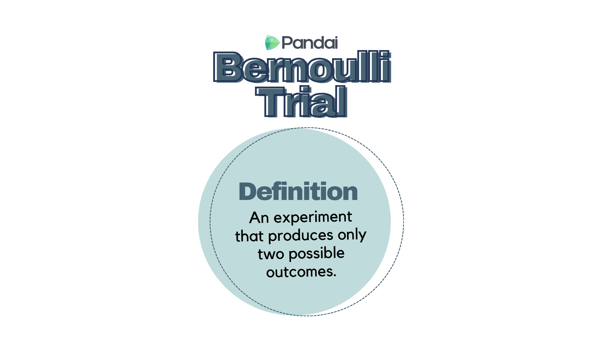
| Characteristics of Bernoulli Trials |
- There are only two possible outcomes, namely 'success' and 'failure'.
- The chances of ‘success’ are always the same in every trial.
- If the probability of 'success' is given by \(p\), then the probability of 'failure' is given by \((1-p)\) where \(0 \lt p \lt 1\).
- The discrete random variable \(X=\{0,1\}\), where \(0\) represents 'failure' and \(1\) represents 'success'.
|
|
| |
| Binomial Random Variable |
| A binomial random variable is the number of success \(r\) from \(n\) similar Bernoulli trials in a binomial experiment. The probability distribution of a binomial random variable is known as a binomial distribution. |
|
| |
| Probability of an Event for Binomial Distribution |
| Formula of Binomial Probability Function for \(X\) |
\(P(X=r)={}^nC_rp^rq^{n-r}\), \(r=1,2,3,...,n\)
|
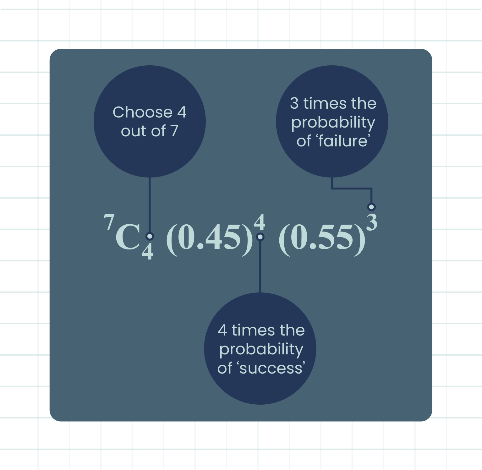
| Explanation for the Formula's Example, \({}^nC_rp^rq^{n-r}\) |
|
| Formula of Total Probability for the Random Variable \(X\) |
\(\sum_{i=1}^n P(X=r_i)=1\)
|
|
| |
| Formula of Expected Value or Mean, \(\mu\) |
\(\mu=\dfrac{\sum_{r=0}^n rP(X=r)}{\sum_{r=0}^n P(X=r)}\)
or
Mean, \(\mu=np\) |
|
| |
| Variance and Standard Deviation |
| Formula of Variance, \(\sigma^2\) |
\(\sigma^2=npq\)
|
| Formula of Standard Deviation, \(\sigma\) |
\(\sigma=\sqrt{npq}\)
|
|
| |
| Example \(1\) |
|
A shelf contains \(6\) identical copies of chemistry reference books and \(4\) identical copies of physics reference books. \(3\) copies of the physics reference books are taken at random from the shelf one after another without replacement.
State whether this probability distribution is a binomial distribution or not. Explain.
|
|
\(P(\text{getting the 1st copy of physics reference book)}\\ = \dfrac{4}{10}= \dfrac{2}{5}.\)
\(P(\text{getting the 2nd copy of physics reference book)}\\ = \dfrac{3}{9}= \dfrac{1}{3}.\)
\(P(\text{getting the 3rd copy of physics reference book)}\\ = \dfrac{4}{8}= \dfrac{1}{4}.\)
The probability of getting a copy of the physics reference book in each trial changes and each outcome depends on the previous outcome.
Thus, it is not a binomial distribution.
|
|
| |
| Example \(2\) |
|
The probability that it rains on a certain day is \(0.45\). By using the formula, find the probability that in a particular week, it rains.
| (a) |
exactly \(4\) days, |
| (b) |
at least \(2\) days. |
|
|
Let \(X\) represent the number of rainy days.
Given \(n = 7\), \(p=0.45\) and \(q = 0.55\).
(a)
\(\begin{aligned} P(X=4) &= \ ^{7}C_{4}(0.45)^4(0.55)^3\\ &= 0.2388. \end{aligned}\)
(b)
\(\begin{aligned} P(X \geqslant 2) &= P(X=2) + P(X=3)+ P(X=4)+P(X=5)+P(X=6)+P(X=7)\\\\ &= 1-[P(X=0)+P(X=1)]\\\\ &= 1- [\ ^{7}C_{0}(0.45)^0(0.55)^7 + \ ^{7}C_{1}(0.45)^1(0.55)^6]\\\\ &= 1-0.0152-0.0872\\\\ &=0.8976 .\end{aligned}\)
|
|
| |
| Example \(3\) |
|
Emma did a survey on the percentage of pupils in her school who use school buses to come to school. It is found that \(45\%\) of pupils from her school use school buses. A sample of \(4\) pupils is randomly selected from the school.
| (a) |
Construct a binomial probability distribution table for the number of pupils who use school bus. |
| (b) |
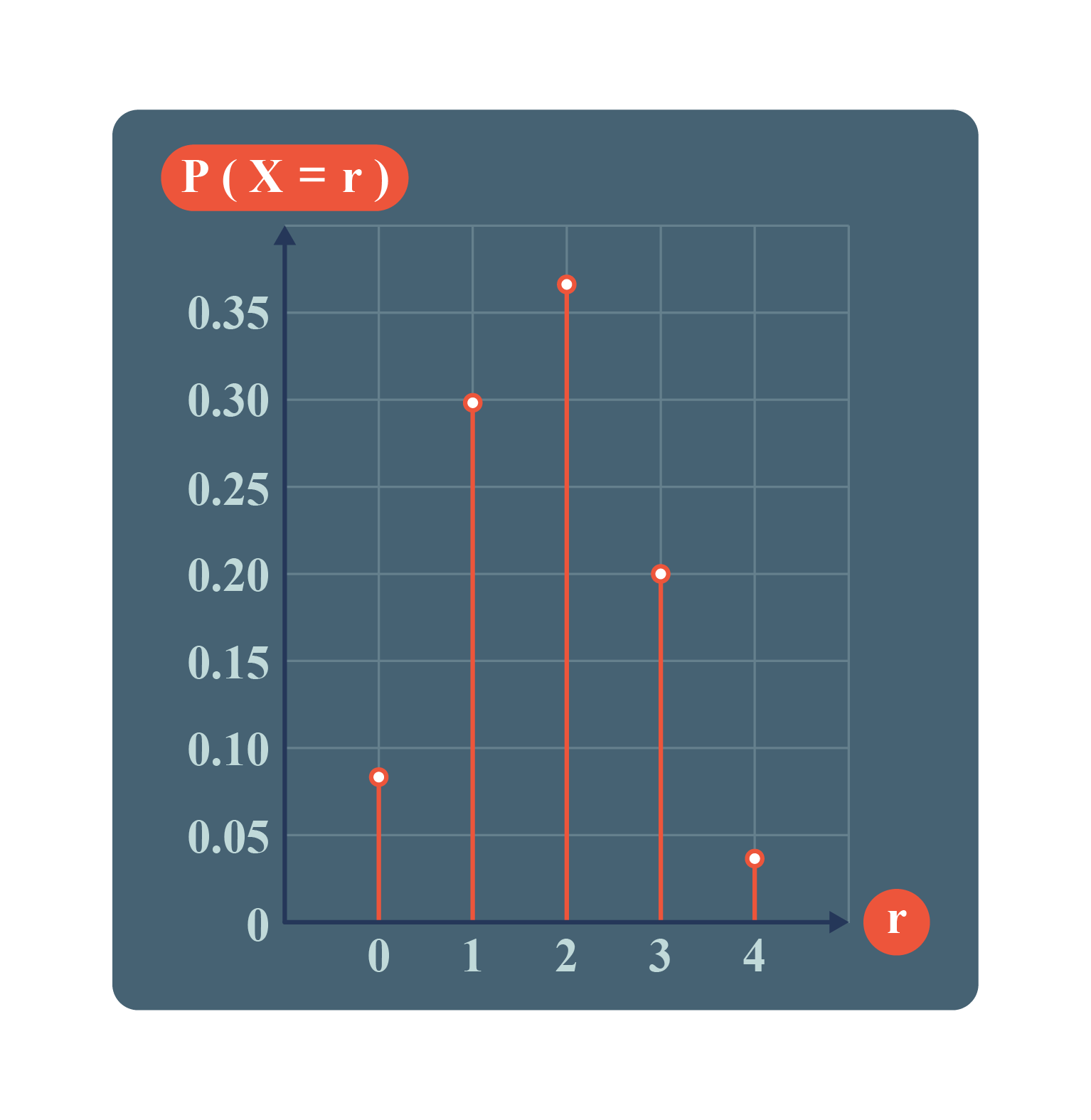
Draw a graph for this distribution. |
| (c) |
From the table or graph, find the probability that |
| |
| (i) |
more than \(3\) pupils come to school by school buses, |
| (ii) |
less than \(2\) pupils use school buses. |
|
|
|
Let \(X\) epresent the number of pupils who use school buses.
Then, \( X = \lbrace 0, 1, 2, 3, 4\rbrace\).
Given \(n=4\), \(p=0.45\) and \(q=0.55\).
| \(X=r\) |
\(P(X=r)\) |
| \(0\) |
\(^{4}C_{0}(0.45)^0(0.55)^4 = 0.0915\) |
| \(1\) |
\(^{4}C_{1}(0.45)^1(0.55)^3 = 0.2995\) |
| \(2\) |
\(^{4}C_{2}(0.45)^2(0.55)^2 = 0.3675\) |
| \(3\) |
\(^{4}C_{3}(0.45)^3(0.55)^1 = 0.2005\) |
| \(4\) |
\(^{4}C_{4}(0.45)^4(0.55)^0 = 0.0410\) |
|
|
|
| (i) |
\(\begin{aligned} P(X\text{ > }3) &= P(X=4)\\ &=0.0410 .\end{aligned}\) |
| |
|
| (ii) |
\(\begin{aligned} P(X\text{ < }2) &= P(X=0) + P(X=1)\\ &=0.0915+0.2995\\ &=0.3910. \end{aligned}\) |
|
|
| |
| Example \(4\) |
|
A study shows that \(95\%\) of Malaysians aged \(20\) and above have a driving license.
If \(160\) people are randomly selected from this age group, estimate the number of Malaysians aged \(20\) and above who have a driving license.
Then, find the variance and the standard deviation of the distribution.
|
|
Given \(p=0.95\), \(q=0.05\) and \(n=160\).
\(\begin{aligned} \text{Mean, } \mu&=np\\ &=160\times 0.95\\ &= 152. \end{aligned}\)
\(\begin{aligned} \text{Variance, } \sigma^2 &=npq\\ &=160\times 0.95 \times 0.05\\ &= 7.60. \end{aligned}\)
\(\begin{aligned} \text{Standard deviation, } \sigma&=\sqrt{npq}\\ &=\sqrt{7.60}\\ &= 2.76. \end{aligned}\)
|
|
| |